
A note on framing before the diagrams. cislunar-sim is not a service architecture. It is a scientific computing library: imported by a researcher in a script or notebook, exercised by CI on every push, and distributed through PyPI. The two diagrams below therefore describe dependency boundaries, not runtime infrastructure.
The same engineering disciplines that matter in production systems (explicit interfaces, reproducible behavior, and validation claims that match reality) matter here as well. A spacecraft simulator simply makes them unusually easy to inspect.
Neither GMAT Nor Orekit Was Built to Be Read
cislunar-sim propagates a spacecraft from low Earth orbit through cislunar space under a physically realistic force environment: Earth’s J2 oblateness, an eight-mascon lunar gravity model derived from GRAIL data, third-body perturbations from the Sun and Moon, atmospheric drag, solar radiation pressure on a sail, eclipse-driven power constraints, and thrust from either an ion engine or a solar sail. It then steers through that environment toward a target orbit using a feedback guidance law, not a learned policy.
The library’s own positioning, stated plainly in its README, is a Python-native alternative to GMAT’s XML configuration and Orekit’s JVM dependency. That gap is real. Both tools are mature and independently validated. Neither is something a research engineer can install with pip and read start to finish in an afternoon.
The headline validation claim is just as plainly stated: the physics engine achieves under 0.05 percent SMA error against SGP4-propagated LightSail 2 states, using bundled TLEs, reproducible from a fresh clone. That is the sentence worth pressure-testing, because it is also the sentence a skeptical reader goes straight to the repository to check first.
Two Kinds of Dependency
cislunar-sim has no runtime footprint in the usual sense. There is no service to page and no client to authenticate. Its two consumers are a research or mission engineer running a script or notebook, and a CI pipeline running the test and benchmark suite on every push, and both pull the same package from PyPI.
What the traditional external-systems box in a context diagram looks like for a physics library turns out to matter more than the box itself. It splits cleanly into two categories, and the split is the point.
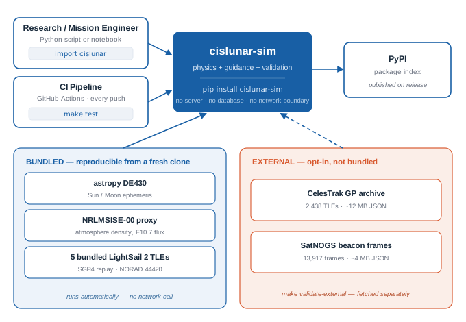
Three data dependencies are bundled and require no network access: Sun and Moon ephemeris
from astropy’s DE430 kernel, atmosphere density from an NRLMSISE-00 proxy driven
by F10.7 solar flux, and five historical LightSail 2 TLEs used for the orbit-replay
comparison. Running make test from a fresh clone exercises all of it,
including the headline SMA-error number, without touching the network.
Two dependencies are explicitly out of the repository: the full CelesTrak GP-history
archive, roughly 12 MB of JSON across 2,438 TLEs, and SatNOGS beacon frames, roughly
4 MB covering eclipse timing and attitude rates. These feed the deeper
cross-checks, the B* drag-swing ratio, eclipse-timing residuals, and the body-rate
envelope, and they sit behind a separate make validate-external target
with its own acquisition instructions. That boundary is deliberate. A test suite that
depends on a 12 MB external archive to pass its core checks is a test suite that
occasionally fails for reasons that have nothing to do with the code under test.
Keeping the reproducible claim and the deeper claim in separate buckets means the
reproducible one never depends on infrastructure outside the repository.
Three Layers, One Direction
The module layout is a clean three-way split: physics, guidance, and validation. Plenty of codebases have three folders. What makes this one worth diagramming is not that the split exists but which direction the dependencies run.
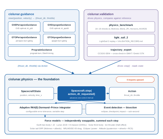
Physics has no import of guidance or validation. It does not know either package exists.
Guidance imports physics to read SpacecraftState and construct an
Action. Validation imports physics to drive it, and sits beside guidance
without depending on it. That asymmetry is the whole design. A bug in a guidance law can
never corrupt the state propagation underneath it, and a change to a guidance law never
requires touching the integrator, the force models, or the validation harness that
proves they are correct.
The Integrator Is Ordinary on Purpose
The integrator is an adaptive Dormand-Prince RK4(5) pair, the same embedded Runge-Kutta family used across general-purpose ODE solvers, chosen for adaptive step control over a fixed-step or symplectic scheme. Force models are independently swappable and summed each step: two-body plus J2 for Earth, J2 and J3 plus an eight-mascon GRAIL model for the Moon, third-body perturbation for the Sun, a Hall-effect ion thruster model with a 60-second warmup delay that actually matters for short burns, McInnes-model solar-sail radiation pressure with albedo, and an NRLMSISE-00 drag proxy.
Event detection, eclipse entry and exit, checkpoint arrival, surface impact, runs as a bisection search for zero-crossings between accepted integrator steps, resolving to sub-second precision without forcing the integrator onto a fixed grid. That precision matters specifically for eclipse-gated ion thrust: get the eclipse boundary wrong by a few seconds across thousands of orbits and the propellant budget drifts in ways that are easy to miss and expensive to unwind later.
Guidance Cannot Reach Into Physics
The interface between the two layers is two tuples. A guidance law receives position and
velocity, and returns a thrust direction and a throttle. Spacecraft.step
does not know or care which guidance law produced the Action it is holding.
It executes whatever it is given.
thrust_dir, throttle = guidance.steer(sc.state.position, sc.state.velocity)
sc.step(
    Action(attitude_dir_cmd=thrust_dir, thrust_dir=thrust_dir, throttle=throttle),
    dt_requested=60.0,
)
That is not incidental encapsulation. Because physics does not know guidance exists, the guidance laws are interchangeable: five of them can be tested against one physics engine, instead of trusting five separate physics-plus-guidance systems independently.
Five concrete guidance laws ship in the repository, ranging from GVE-based feedback control to a prograde-burn baseline, and every one of them implements that same contract. None involves a training loop: state goes into a feedback function, the function returns a direction and a throttle, and the loop repeats. There is no policy to train and no learned behavior to trust on inputs it never saw. The specific control laws, including the Q-law formulation and its GVE and GTO variants, are documented in the repository.
A Validation Record That Names Its Own Limits
The validation record is more specific than a marketing sentence, and more honest than most.
The headline SMA-error number, 0.0112 percent in the most recent re-validation run, comes from replaying archival LightSail 2 TLEs through SGP4 to build an hourly reference trajectory, then propagating the same intervals through cislunar-sim’s full force model and comparing. The record is explicit about what that number does and does not establish: SGP4 propagation carries its own error, on the order of one to two kilometers a day for a low orbit, so this comparison measures agreement between the physics engine and SGP4, not agreement between the physics engine and raw telemetry. That is a meaningfully narrower claim than most validation write-ups make, and it is stated as a caveat in the library’s own documentation rather than left for a reader to discover independently.
What the validation record actually shows
| Result | Value | Source |
|---|---|---|
| SMA error (1-day archival epoch) | 0.0112% | bundled TLEs, make test |
| Radial error | 0.007% of orbital radius | bundled TLEs, make test |
| Sail force vs. McInnes (IKAROS params) | within 1% | bundled, make test |
| B* swing ratio, sail vs. passive | 0.231 observed vs. 0.228 predicted | CelesTrak archive, make validate-external |
| Eclipse entry timing | +3.7s mean, 19.5s std (77 usable windows) | SatNOGS archive, make validate-external |
The eclipse-timing row is described in the library’s own record as promising rather than conclusive, limited by beacon cadence rather than by the shadow model.
The strongest single result does not come from the bundled data at all. It comes from
splitting two and a half years of CelesTrak history into a sail-deployed window and a
sail-furled window and comparing the ratio of fitted B* drag terms: 0.231 observed
against 0.228 predicted from the published LightSail 2 mission results, a result that
requires the external archive, which is exactly why it sits behind
make validate-external instead of the default test suite.
The record also documents where it falls short. Eclipse-timing validation against SatNOGS beacon frames is described in the library’s own documentation as promising, blocked by beacon-cadence heterogeneity: 77 usable transition windows out of several thousand frames, entry-timing residuals centered near zero but with roughly 20 seconds of scatter at 45-second beacon cadence. Not yet a precise validation, and the documentation says so rather than rounding up.
A recent re-validation run also disclosed a real bug: the solar-sail radiation-pressure model had been applying the absorptivity term to the wrong part of the force equation, understating net SRP force. The fix increased net SRP force by roughly 72 percent for LightSail 2’s sail parameters. The correction increased physical fidelity. It did not materially change the library’s principal validation claims. That is exactly what a validation record is supposed to reveal.
What This Deliberately Does Not Do
A few decisions here will draw questions from people who work in orbital mechanics professionally, and they are worth addressing directly instead of leaving them as unstated defaults.
RK4(5) over a symplectic integrator. Long-duration propagation is a classic case for symplectic integrators, which conserve a shadow Hamiltonian and avoid the secular energy drift that general-purpose adaptive integrators can accumulate over very long horizons. cislunar-sim does not use one. Most of what this library targets is transfer trajectories measured in days to weeks, not multi-decade propagation, and an adaptive Dormand-Prince pair with tight tolerances is accurate enough over that horizon while being far simpler to extend. Adding a force model to a symplectic scheme usually means re-deriving the splitting; adding one here means writing an acceleration function. A use case needing multi-decade fidelity would be a real argument for a second integrator option, not a reason the first choice was wrong.
Q-law over indirect optimal control. GVE-based Q-law is a feedback law. It does not solve a two-point boundary value problem and does not require an initial costate guess, so it does not fail to converge the way indirect shooting methods can on a poor guess. It is also not provably time-optimal the way a correctly converged indirect solution is. For a simulation and guidance-research tool, where robustness and the ability to re-target mid-transfer matter more than shaving the last few percent off transfer time, that is the right trade. For a mission-design tool computing a single trajectory against a fixed, unforgiving propellant budget, it might not be.
Pure Python over a compiled core. GMAT and Orekit both made a different bet here for a reason: raw propagation speed matters when running large Monte Carlo dispersion sets. cislunar-sim’s answer is that a seven-day GTO periapsis raise and a five-day drag-decay case each complete in under a minute on ordinary hardware, which is fast enough for the research and validation use case this library targets. It is not fast enough to replace a compiled propagator in a Monte Carlo campaign with tens of thousands of runs, and it is not trying to be.
What is out of scope for this release. No N-body dynamics beyond Earth, Moon, and Sun. No relativistic corrections. No flight-software emulation: guidance laws run in the simulation loop, not on an emulated flight computer. Attitude dynamics are modeled, quaternion rigid body, reaction wheels, cold-gas RCS, but attitude is not yet a guidance target in its own right, only a consequence of the commanded thrust direction. Each of these is a real feature someone will eventually want. None of them was free to skip, and none was skipped by accident.
Software engineering often treats architecture as something inferred from source code after the fact. Scientific software benefits from making those boundaries explicit. cislunar-sim is one example, but the principle is broader: if validation claims, dependency boundaries, and module responsibilities are understandable from the outside, they become easier to trust, and easier to improve.
A companion piece on CTO Insights, Models Converge on Consensus, Not Correctness, examines a specific episode from building this: what happened when the guidance problem was handed to a language model, repeatedly, and the model kept reaching for the same answer regardless of how the question was framed. That piece is about the model. This one is about the machine it was asked to help build.
cislunar-sim is available now on GitHub and PyPI under the MIT license.